13 Quick Linear Regression

13.1 Quick Linear regression using Loblolly

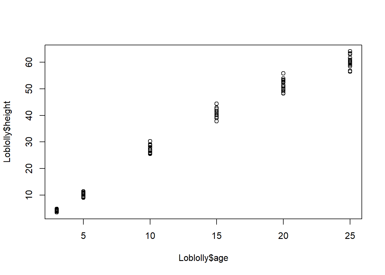
1. load Loblolly and create a scatter plot of the data so plot so that age is the independent variable and height is the dependent variable.

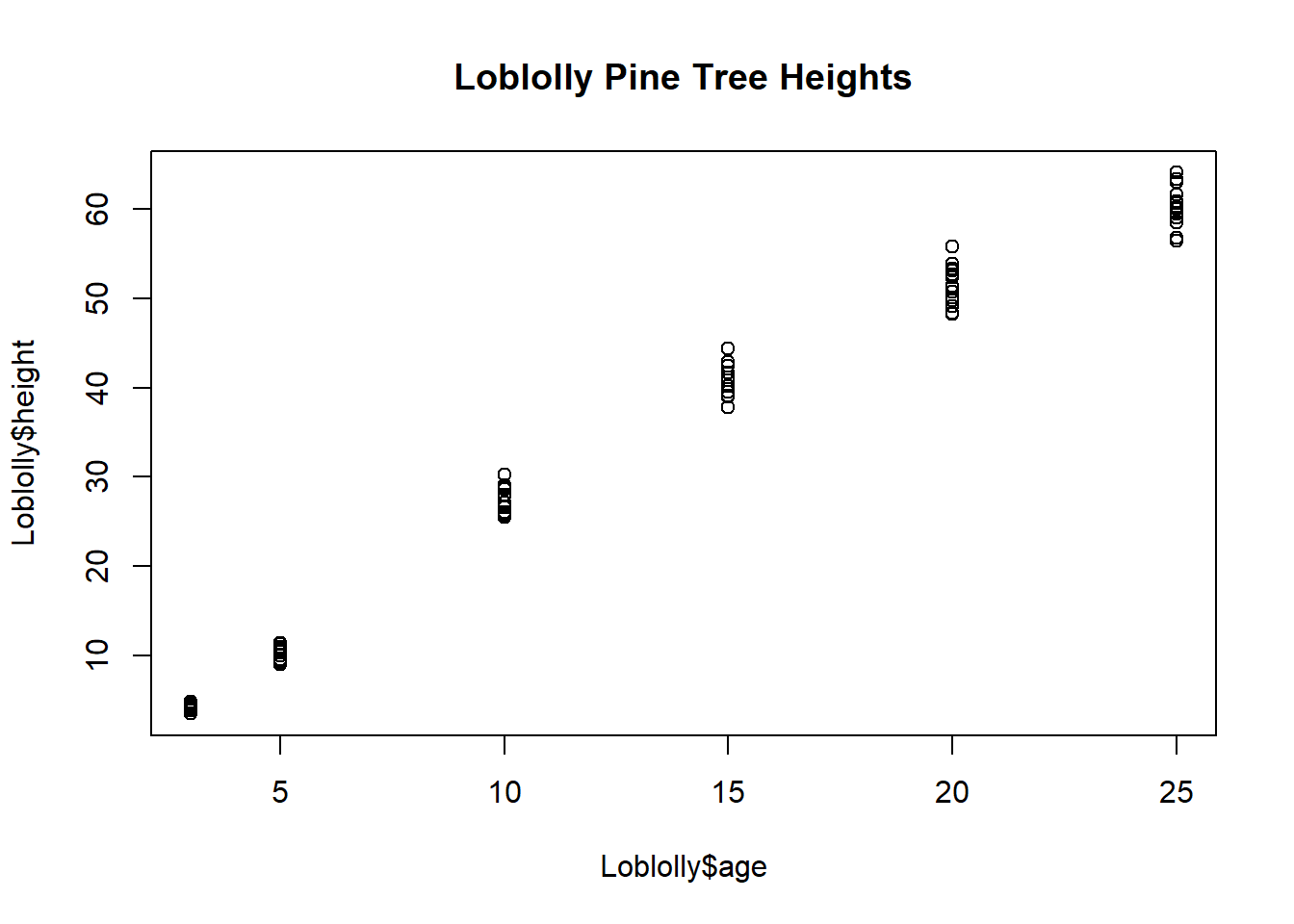
2. Notice that R automatically labeled the x- and y-axes, but we also want our scatter plot to have a main title. To add a title, use the command title(main = “Loblolly Pine Tree Heights”).

3. To find a linear model that relates the age and height of the loblolly pine trees, we will use the command fit1<-lm(Loblolly$height~Loblolly$age).

Think of lm(Loblolly$height~Loblolly$age) as the slope-intercept form (y=mx+b).

4. To see the model, type fit1

fit1 <- lm(Loblolly$height~Loblolly$age)
fit1
#> 
#> Call:
#> lm(formula = Loblolly$height ~ Loblolly$age)
#> 
#> Coefficients:
#>  (Intercept)  Loblolly$age  
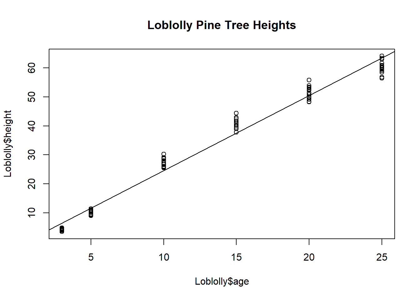
#>       -1.312         2.591

5. Now we want to add the graph of this line of best fit to our scatter plot. To do this, use the command abline(fit1). .

9. The final piece of information we want about our data is the correlation of the age and height of the Loblolly pine trees. To find the correlation coefficient, use the command cor(Loblolly$height, Loblolly$age)

#> [1] 0.9899132
#> 
#>  Pearson's product-moment correlation
#> 
#> data:  Loblolly$height and Loblolly$age
#> t = 63.272, df = 82, p-value < 2.2e-16
#> alternative hypothesis: true correlation is not equal to 0
#> 95 percent confidence interval:
#>  0.9844505 0.9934631
#> sample estimates:
#>       cor 
#> 0.9899132

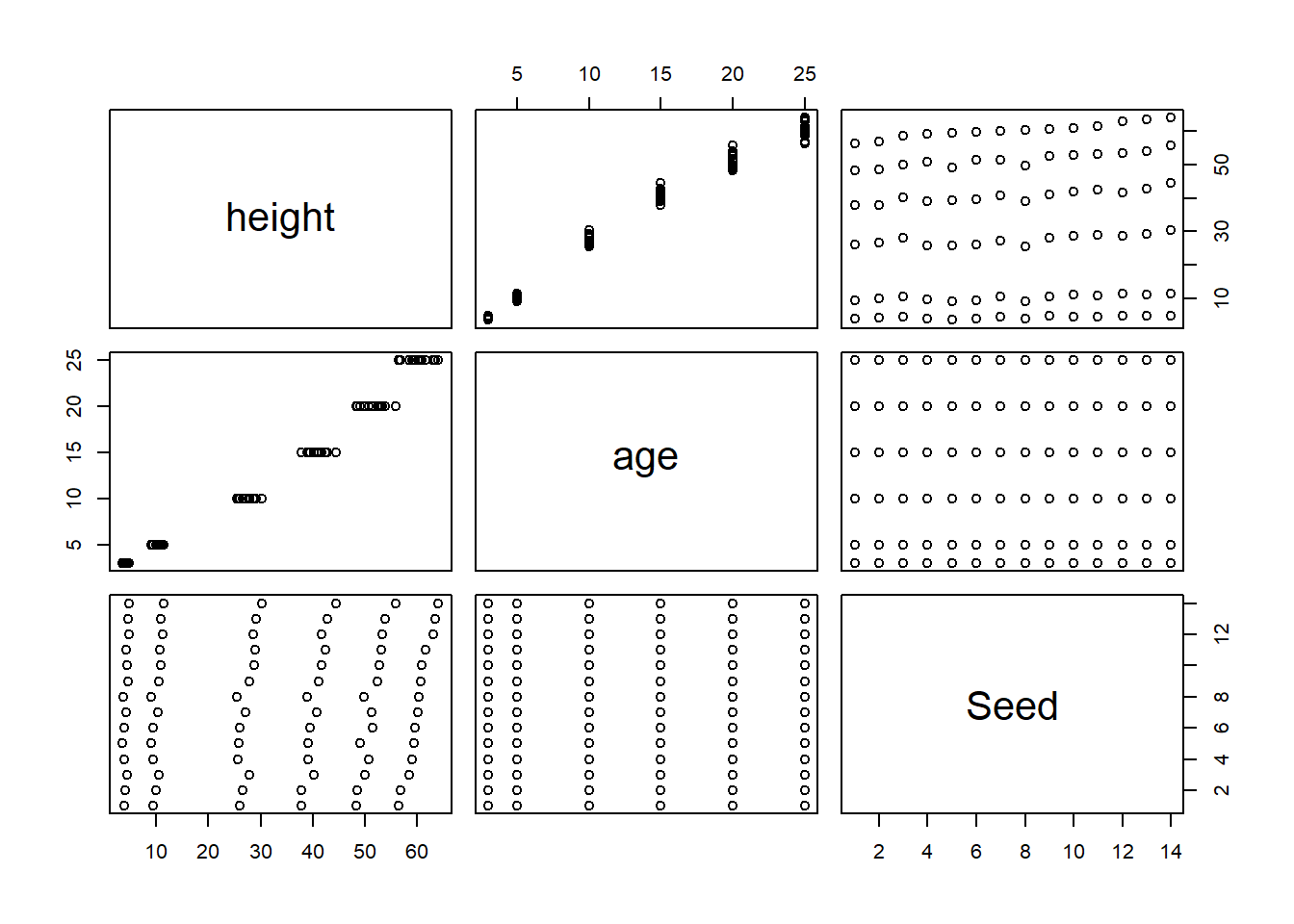
10. What does this command do and mean: plot(Loblolly)?